
Reviewed captions introduce indexed matrix dimensions, corresponding-entry addition and scalar operations.
Give every number an address
A matrix is more than a collection of numbers: its arrangement carries information. Imagine two workshop sites, each tracking three kinds of supplies. Put sites in rows and supplies in columns. The entry in row two, column three now has a precise meaning. If you transpose those labels mentally, a correct arithmetic operation can still answer the wrong practical question. Write the row and column labels before you calculate.
The linked introductory video explains row-first dimensions, indexed entries, corresponding-entry addition and scalar multiplication. We read its captions from the opening through 650 seconds. The workshop example, calculations and comparison below are original teaching material. The caption track does not reliably preserve the layout of every displayed matrix, so this article does not reconstruct the source diagrams or claim full audiovisual review.
Build and read the workshop table
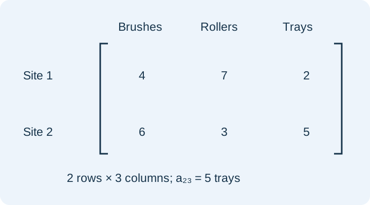
Our inventory matrix A has first row [4, 7, 2] and second row [6, 3, 5]. The columns represent brushes, rollers and trays, in that order. There are two rows and three columns, so A has dimensions 2 by 3. Entry a23 equals 5: the second site holds five trays. Entry a12 equals 7: the first site holds seven rollers. These are addresses, not multiplication instructions.
The original figure places row labels to the left and supply names above the columns. Use it to locate a21 before checking: the value is 6. Moving one position right gives a22=3, while moving up gives a11=4. This small spatial check helps distinguish a mistaken row-column swap from an arithmetic mistake. A matrix with six entries could have several shapes; the number of entries alone does not determine its dimensions.
Add matching information
A delivery matrix B has rows [1, 2, 4] and [3, 1, 2], using the same site and supply order. After delivery, the inventory A+B has rows [5, 9, 6] and [9, 4, 7]. Each new count combines exactly one original inventory count with its matching delivery count. For example, the second site now has 5+2=7 trays. It would be meaningless to add that tray count to a first-site brush delivery.
Both matrices must have the same dimensions for entrywise addition. In a contextual model, their labels and units must also agree: a count of trays should not be silently added to a cost in dollars. Equal shape is a mathematical requirement, while matching meaning is an additional modeling requirement. If the delivery table lists supplies in another order, reorder it consistently before performing the addition.
Separate scaling from subtraction
Suppose a planning sheet requests the numerical matrix 2A−B. Its first row is [7, 12, 0] because 2(4)−1=7, 2(7)−2=12 and 2(2)−4=0. Its second row is [9, 5, 8] because 2(6)−3=9, 2(3)−1=5 and 2(5)−2=8. The scalar 2 applies to A only. It does not apply to the subtracted matrix unless parentheses explicitly say so.
Compare 2(A−B): its rows are [6, 10, −4] and [6, 4, 6]. The difference is systematic rather than random. The second expression also doubles B before subtraction. A negative entry is valid in a numerical matrix; interpreting it as an actual stock count would require a new explanation, such as a shortage. Do not confuse algebraic validity with the feasibility of a physical interpretation.
Know when a new operation begins
Matrix multiplication is a different operation from entrywise addition or scalar multiplication. It uses compatible inner dimensions and row-column products. You should not multiply corresponding entries merely because that worked for addition. A determinant is different again: it applies to a square matrix and produces one number. These extensions are introduced in our linked practice lesson, but they are not presented here as claims from the reviewed introductory video.
For an original two-by-two example C=[[4,2],[3,5]], the determinant is 4 times 5 minus 2 times 3, or 14. The result is neither the sum of all four entries, 14 by coincidence here, nor a general rule to add the entries. Change the lower-right entry from 5 to 6: the determinant becomes 18, while the entry sum becomes 15. The contrast reveals why a single agreeing example cannot validate a method.
Retrieve one result, then explain it
Without recalculating a whole matrix, find entry (1,2) of 3A−B for the original inventory and delivery matrices. That entry is 3 times 7 minus 2, which equals 19. The corresponding entry of 3(A−B) would instead be 15. State which matrix is scaled and identify the exact addressed entries. A compact explanation of that distinction is more useful than an unexplained list of matrix answers.
Finally, check dimensions, positions, signs and context separately. Dimensions establish whether an operation is defined; positions identify the correct data; signs determine the numerical result; context determines whether that result answers the application. This sequence supports ACT number-and-quantity practice while leaving fuller matrix systems, inverses and geometric transformations for later study. It is a focused companion, not a complete matrix course.
PAUSE & TRYWhat is entry(1,2) of3A−B for the original matrices?Reveal explanation
19:3×7−2.
Turn the idea into practice.
A fresh set will help you use the relationship with different numbers.
Practice this skillEvidence & editorial note
Freshly acquired English captions. Original examples and diagrams; no transcript republication. Read 0–650 seconds; determinant example is an original extension beyond these introductory operations.
Brief source synopsis and independently authored instructional companion.
Caption track SHA-256: 0298a1f6dedaa61e4f4e9524c4a6809de27e4b73d3f12a5b1a79607c569bbf54
Source segment references are retained in the catalog. Full captions remain in the local research archive.