Translate data into log space. · AP Precalculus

A change of coordinates can expose a pattern

Suppose positive measurements at times0,2 and4 are10,100 and1000. The successive differences90 and900 are not constant, but the successive ratios are both ten. Now replace each measured output y by its base-ten logarithm L. The same observations become(0,1),(2,2) and(4,3), which lie on a straight line. This transformed display is a semi-log plot because the horizontal variable remains untransformed while the vertical coordinate is logarithmic. The original data have not changed; their representation has. A straight line on this display therefore needs a different interpretation from a straight line on ordinary axes.

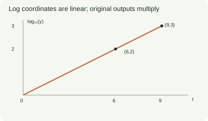
The overview figure belongs to the later interpolation example with log₁₀(y)=t/3. The opening example instead uses log₁₀(y)=1+t/2; keep their different initial values separate.

Name the vertical coordinate before using its slope

The slope in the transformed coordinates is(3−1)/(4−0)=1/2. The intercept is1, so L=1+t/2. Since L=log₁₀(y), exponentiating gives y=10^(1+t/2)=10×10^(t/2). The initial output is10, and the multiplier over two time units is10. The multiplier over one time unit is√10. Saying that the original output rises by one half per time unit would misuse the slope: one half is the increase in log₁₀(y), not the increase in y. Always write the axis variable beside the equation when moving between these two representations.

Use a different base without changing the model

A different original example uses log₂(y)=6−2t. The intercept6 corresponds to y(0)=64, not six. Increasing t by one decreases the logarithm by two, so the original output is multiplied by2^(−2)=1/4. At t=1 the output is16, at t=2 it is4, and at t=3 it is1. The negative line slope describes positive decay. It does not make y negative. A logarithmic vertical coordinate can be negative when the original output lies between zero and one; for example, log₂(1/4)=−2. The original output must still remain positive.

Interpolate in the representation actually supplied

On a straight-line display of log₁₀(y) against t, suppose the points are(0,0) and(6,2). The line has slope1/3. To find when y=1000, first convert the target into log coordinate3. Solving t/3=3 gives t=9. Interpolating directly to a vertical value1000 on this display would confuse the original output with its logarithm and produce a meaningless time. The figure marks the three transformed points. Their original outputs are1,100 and1000. The last prediction is an extrapolation beyond the two supplied times, so a real application would need evidence that the same exponential relationship continues.

Open full-size diagram ↗

Compare model assumptions with observed data

A logarithmic transformation can reveal an approximately linear pattern, but it does not prove that a physical process is exponential. Measurement error, changing conditions and limited observation ranges still matter. Check whether the time intervals are equal before comparing simple ratios. If the observed original outputs are10,100 and900 instead of1000, the last point no longer lies exactly on the predicted log line. A residual in original output units differs from a residual in logarithmic units. Choose the scale according to the modeling question, and state it. This companion uses exact illustrative data rather than presenting a fitted model as an empirical finding.

Connect the plot to inverse questions

The source’s selected early captions show how initial and later observations determine an exponential expression and how logarithms help isolate its constant. The semi-log diagram here is an original extension of that modeling idea; it is not claimed to appear in the selected video segment. Once y=A b^t has been established, solving for time gives t=log_b(y/A), provided A and y are positive and b is positive but not one. For the first example, reaching y=10000 means10^(t/2)=1000, so t/2=3 and t=6. Check the answer against the two-unit factor: three multiplications by ten carry10 to10000.

A written transfer check

A new display gives log₁₀(y)=2−t/4. Identify the initial output, the factor over four time units and the time when y=1. The answers are100,1/10 and8 respectively. To justify them, exponentiate the intercept, translate a change of−1 in the log coordinate into a factor of one tenth, and set the target log coordinate to zero. Explain why y never reaches zero at a finite time in this positive exponential model. These are original teaching questions. The existing source captions are deliberately reused for a distinct representation lesson; later calculus material is excluded, and full audiovisual and educator review remain pending.