
The inspected captions explain class widths, frequency densities and histogram construction. The examples and illustrations below are independently authored.
Start with a grouped continuous variable
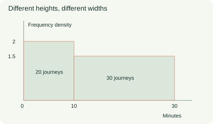
A histogram displays a numerical variable grouped into intervals. The width of a bar follows the class boundaries on the horizontal scale, so unequal class widths remain visibly unequal. Imagine an original table of journey times: 20 journeys last from 0 up to 10 minutes, and 30 journeys last from 10 up to 30 minutes. The first interval has width 10 and the second width 20. A diagram that gives both bars the same arbitrary width would lose part of the information. Before drawing anything, calculate each upper boundary minus its lower boundary and keep the class interval convention clear.
Turn counts into heights
Histogram height is frequency density, defined as frequency divided by class width. The first class therefore has density 20/10=2 journeys per minute of class width. The second has density 30/20=1.5. The second bar is lower, even though it represents more journeys. Its extra width compensates for the smaller height. Multiplying each height back by its width recovers the original counts: 2×10=20 and 1.5×20=30. This reversible calculation is a useful check on both the table and the drawing. The figure uses an actual numerical scale so that its bar areas preserve the same comparison.
Explain why area matters
Area equals width times height. Replacing height by frequency density makes a bar’s area equal its frequency in data-coordinate units. That is why two bars can have equal areas and different heights. In another original example, a width 4 class with density 3 and a width 6 class with density 2 each represents 12 observations. Looking only at height would wrongly suggest that the first class contains more observations. Equal-width bar charts often encourage that habit, so unequal-width histograms require a deliberate change of interpretation. The vertical axis should be labeled frequency density, not merely frequency, whenever those heights are used.
PAUSE & TRYDo width 4,density 3 and width 6,density 2 bars represent equal counts?Reveal explanation
Yes:both have area and frequency12.
Recover a missing table entry
Suppose a histogram bar begins at x=3 and ends at x=9, with density 5. Its width is 6 and its frequency is 30. If instead its frequency were given as 30 and its density as 5, division would recover the width 6. None of these operations requires the lower boundary itself to be zero. A common mistake is to multiply density by the upper boundary 9, forgetting that the bar begins at 3. Another is to divide density by width, reversing the relationship. Label the three quantities frequency, width and density before choosing the operation, then check by multiplying width and density.
Estimate a count inside one class carefully
A class 10≤x<30 contains 20 observations. To estimate the number below 15 within that class, a usual assumption is that observations are spread uniformly across the class. The interval 10≤x<15 occupies one quarter of its width, so the estimate is 5 observations. This is an estimate because the grouped table does not reveal the individual values. It is possible for the actual count in that subinterval to differ substantially. The bar’s constant height represents the grouped model; it does not establish that the underlying observations were literally evenly spaced. State the assumption whenever a question asks you to divide a class internally.
PAUSE & TRYA width 20 class contains 20 observations. Under uniform spread, how many are estimated in its first 5 units?Reveal explanation
5observations, one quarter of the class frequency.
Draw the scale before the rectangles
Choose a horizontal scale that preserves every class boundary and a vertical scale that includes the largest density. Draw each rectangle from its lower boundary to its upper boundary, using the calculated density as its height. Adjacent continuous classes meet; unexplained decorative gaps would suggest a different representation. A written solution should show the density calculations as well as the finished chart, so a scale error can be distinguished from an arithmetic error. The inspected video captions explain this construction sequence. The journey-time data, equal-area contrast and missing-frequency exercise in this article are independently authored examples.
Transfer and source limitations
For a transfer check, two classes are 0≤x<5 with frequency 15 and 5≤x<20 with frequency 30. Their densities are 3 and 2. The second class has twice the count but only two thirds the height, since it is three times as wide. Explain that result using areas before considering the drawing finished. A second check asks whether the tallest bar always represents the most frequent class; the answer is no when widths differ. Selected actual captions were read through the drawing summary, and the illustrated calculations were checked separately. Full audiovisual and independent educator review are still pending. The source is a GCSE explanation used for a method that is also explicitly included in Cambridge 0580 Extended; it is not described as an official Cambridge video.
Turn the idea into practice.
A fresh set will help you use the relationship with different numbers.
Practice this skillEvidence & editorial note
Actual selected captions read. GCSE teaching method mapped to 0580 Extended; source is not an official Cambridge video. New caption acquisition. Full audiovisual and educator review pending.
Original teaching companion with brief source synopsis.
Caption track SHA-256: 9d40ce20644f3b0d5f1d8bcd1a4621f5f0d00dbb4afc37168edfee004552dc61
Source segment references are retained in the catalog. Full captions remain in the local research archive.