
StatQuest explains why numerical observations are grouped into bins and why bin width changes the visual story. This companion develops independent delay examples and distinguishes descriptive frequency from a validated probability model.
Begin with the measurement, not the software default
A delivery team records twelve delays in minutes: one, two, four, five, six, seven, eight, nine, ten, fourteen, fifteen and nineteen. Each number belongs to a delivery. Before drawing a chart, identify whether a delay measures arrival relative to the scheduled time, departure time or customer request. Those are different variables, even if all are reported in minutes.
The first useful question is descriptive: where do these observed delays lie? A later question might ask whether future deliveries will follow a similar pattern. A chart can inform that later question, but it cannot supply a stable operating process, a representative sample or a large enough dataset by itself. Keep the measurement definition and collection period next to the graph.
Make the boundary convention visible
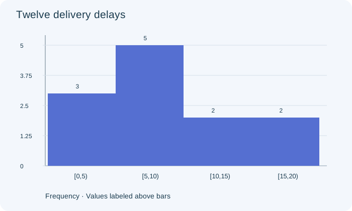
Use equal-width bins from zero to five, five to ten, ten to fifteen and fifteen to twenty minutes, including each left endpoint and excluding each right endpoint. The frequencies are three, five, two and two. The five-minute delay goes in the second bin and the fifteen-minute delay goes in the fourth. Counting either boundary twice would create observations that never occurred.
The original figure shows these four counts. Its vertical axis is frequency, so the tallest bar contains five deliveries. The bars touch because their horizontal intervals are adjacent numerical ranges. A categorical bar chart would use separated categories; ordering categories alphabetically would not give the same numerical continuity. Explain the axes before describing the shape.
PAUSE & TRYHow many recorded delays are at least five but less than fifteen minutes?Reveal explanation
Seven: five from [5,10) and two from [10,15).
Recover only the information the bins retain
The histogram tells us that seven delays lie between five and fifteen under the stated endpoint convention. It does not tell us the exact values within those two bins. If only the histogram survived, replacing every observation by its bin midpoint would produce an estimate of the mean, not an exact recovery of the original mean.
Because we have retained the original list, we can calculate its total as one hundred minutes and its mean as one hundred divided by twelve, or about eight point three three minutes. For the midpoint approximation, multiply the four midpoints by their counts, add to one hundred five, and divide by twelve to get eight point seven five. The discrepancy is information lost through grouping.
Compare a second team on a compatible scale
Suppose a second team records twice as many deliveries in every bin: six, ten, four and four. Its frequency bars are twice as tall, but its relative-frequency distribution is identical. Both teams have one quarter in the first bin, five twelfths in the second and one sixth in each remaining bin. The second team has more observations, not a larger fraction of long delays.
When sample sizes differ, plot relative frequencies or explicitly compare rates. Keep the same boundaries and horizontal scale so a difference in display choices does not masquerade as a difference in performance. If one team measured only morning deliveries and the other included evening congestion, even a visually fair comparison still needs a discussion of collection conditions.
Try another width without shopping for a conclusion
Combining the first two bins gives eight delays below ten minutes; combining the last two gives four delays from ten to twenty. The broad two-bin view is simple, but it hides the peak in the five-to-ten interval. Much narrower bins would reveal more local detail while creating a jagged picture from only twelve measurements. Neither view automatically reveals a uniquely true shape.
Inspect a few reasonable widths and report features that persist. Do not select only the width that makes a favored claim look strongest. For unequal-width histograms, frequency density is needed if bar area is to represent frequency; the equal-width teaching figure avoids that additional complication. An apparent gap or second peak deserves inspection of raw values and relevant subgroups.
Separate a data story from a population promise
The sample is small and may come from one unusual shift. Its largest delay is an observation to investigate, not a reason for automatic deletion. A normal approximation would need further support; the chart alone does not prove a normal population or guarantee tomorrow’s tail probabilities. Changes in routes, staffing or weather can invalidate a model fitted to yesterday’s process.
A defensible written response states the variable and units, describes the observed intervals, compares counts or proportions with the right denominator, and identifies information lost by grouping. Then it distinguishes those sample descriptions from any population claim. The transferable skill is to explain how the display supports a statement, including what remains unknown, rather than merely naming the tallest bar.
Turn the idea into practice.
A fresh set will help you use the relationship with different numbers.
Practice this skillEvidence & editorial note
English automatic captions from 35–201 seconds read in full. The source suggests using histogram shape to inform a probability model; our article adds sampling, stability and validation conditions. No source images, transcript paraphrase or audiovisual review claimed. All examples and figures below are original.
Original worked examples, argument and SVGs; short source map only.
Caption track SHA-256: 0901e65ec82629e90b10639609d409b80090637416e6d1a9f69355db4f333146
Source segment references are retained in the catalog. Full captions remain in the local research archive.