
StatQuest illustrates distributions of repeated sample means from nonnormal populations. This companion uses an independent exact two-point example, then states the finite-sample and moment conditions behind a normal approximation.
Name three distributions before using one theorem
Imagine a machine that independently outputs either zero or two tokens with equal probability. One output is an observation. A batch of four outputs is one sample. The average of those four numbers is one sample statistic. Repeating the entire batch produces a distribution of averages. Keeping these objects distinct prevents an easy but consequential misunderstanding of the central limit theorem.
The population of individual outputs has only two possible values, so it is certainly not a smooth normal distribution. The distribution of a four-output average has five possible values. A histogram built from a thousand simulated batches estimates that second distribution. It is a plot of statistics, not a plot of the original machine outputs.
Calculate a small sampling distribution exactly
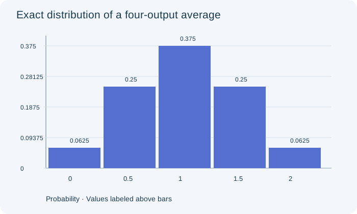
Let K count the two-token outputs in a batch of four. Each of the sixteen equally likely binary sequences determines one batch, and the batch average is K divided by two. Averages zero, one half, one, one and one half, and two therefore have probabilities one sixteenth, four sixteenths, six sixteenths, four sixteenths and one sixteenth.
The original figure displays those probabilities. The middle average is most common because six sequences contain exactly two high outputs. The average distribution already has a central concentration even though the individual distribution places all its mass at the two extremes. It remains discrete and cannot be exactly normal. A smooth approximation should not erase that finite-sample fact.
PAUSE & TRYWhat is the exact probability that the four-output average equals one?Reveal explanation
6/16 = 3/8, from the six sequences containing exactly two high outputs.
Explain the spread in the correct units
For one machine output, the population mean is one token and the population standard deviation is one token. For an average of four independent outputs, the mean remains one while the standard deviation is one divided by the square root of four, or one half token. Averaging makes the statistic less variable; it does not change the spread of individual outputs.
For an average of sixteen outputs, the standard deviation is one quarter token. Increasing the sample size fourfold halves the standard error. This calculation follows from independence and finite variance, not from pretending that the individual outputs are normal. Always state whether a reported spread describes observations or estimates, because both can have the same measurement units.
Distinguish more repetitions from more observations per mean
Suppose a computer draws one hundred batches of four, then ten thousand batches of four. The second run gives a more stable estimate of the five exact probabilities. The target sampling distribution is unchanged because every batch still has four observations. Its standard deviation is still one half token; the simulation has not magically made each mean more precise.
Changing the batch size from four to sixteen does change the sampling distribution. There are more possible averages, less spread and typically a better normal approximation in this bounded example. A simulation report should record both numbers: observations per batch and total batches. A single unlabeled sample-size value makes it impossible to know which source of variation was changed.
Keep the conditions in the theorem
For independent identically distributed observations with a finite population mean and variance, the standardized sample mean approaches a normal distribution as sample size grows. The approximation can be useful at moderate sizes, but its accuracy depends on population shape and on the probability region being estimated. A statement that thirty always suffices is not a universal mathematical rule.
Strong skewness, very rare large values or dependence can make a routine approximation misleading. A finite recorded sample from a Cauchy distribution still has an arithmetic average, but that population lacks the finite moments required by the ordinary theorem used here. Saying that the sample mean cannot be calculated confuses an observed arithmetic operation with a property of the population distribution.
Use the distinction when reporting inference
An approximate normal sampling distribution can support inference about a mean when the design and method conditions are suitable. It does not remove selection bias, make correlated observations independent, or validate every test involving an average. Choosing a t procedure also requires attention to estimating the unknown population spread and to the study design.
For a written transfer check, explain why collecting more machine batches cannot repair a defective simulation that makes successive outputs dependent. The simulation must first represent the intended mechanism. Then more repetitions improve numerical precision. A persuasive answer identifies the distribution, checks assumptions, and explains what changes when the sample size changes, rather than simply invoking the theorem by name.
Turn the idea into practice.
A fresh set will help you use the relationship with different numbers.
Practice this skillEvidence & editorial note
English captions from 66–429 seconds read. The source informally calls finite-sample means normal; this companion says approximately normal when justified. Its Cauchy remark confuses a nonexistent population mean with an observed sample mean, which can be computed; we correct this distinction. The usual CLT used here assumes independent identically distributed observations with finite variance. No full audiovisual review.
Original worked examples, argument and SVGs; short source map only.
Caption track SHA-256: b5702429c1551a5e178339e5f18b3c7d41f8f60eeafb6594443d76f8e27a7122
Source segment references are retained in the catalog. Full captions remain in the local research archive.