
The selected StatQuest segment introduces least-squares residuals and compares variation around a fitted line with variation around the response mean. This companion uses a new three-point teaching dataset to develop those ideas and adds AP-specific interpretation limits.
Begin with a paired measurement
Imagine recording hours spent on one training exercise and the number of tasks completed correctly afterward. Each participant contributes an ordered pair: practice time is x and completed tasks is y. The outcome can vary among people who spend the same time, so a model predicts a typical response rather than guaranteeing a person’s result. The relationship is observational unless time was assigned through an appropriate experimental design.
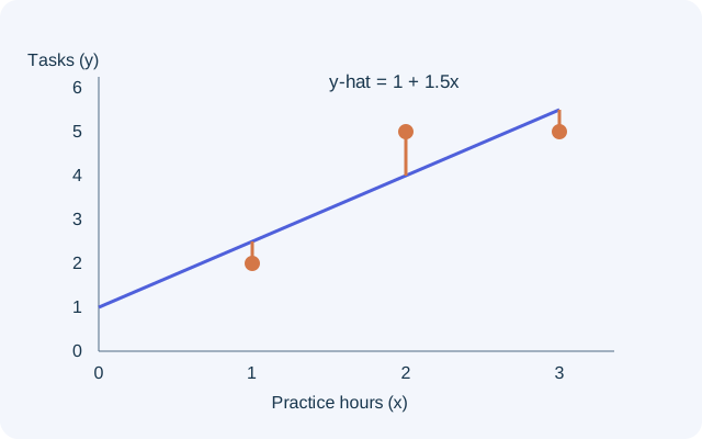
Use the deliberately small teaching dataset (1, 2), (2, 5), and (3, 5). Three observations are enough to demonstrate arithmetic, but they are far too little evidence to validate a useful real-world prediction system. We will keep that limitation visible rather than using an impressive-looking fit statistic as a substitute for data collection. Draw the points before calculating, and keep both axis labels and their units.
Separate the fitted value from the observed value
For these points the least-squares line is y-hat = 1 + 1.5x. At x = 2, the fitted value is 4 completed tasks while the observed response is 5. The residual is observed minus predicted, so it equals 1 task. A positive residual means the model underpredicts this observation. Reversing the subtraction would reverse the interpretation.
At x = 1 the prediction is 2.5 and the residual is −0.5; at x = 3 the prediction is 5.5 and the residual is also −0.5. A model for a count may give fractional predictions because it estimates an average response. That does not mean a particular participant completed half a task. The plotted vertical gaps, measured at fixed x values, represent residuals. They are not the shortest perpendicular distances to the line.
PAUSE & TRYFor y-hat = 1 + 1.5x, what is the residual when x=2 and observed y=5?Reveal explanation
1 task: 5−(1+1.5×2)=1. The model underpredicts.
Explain why the fit uses squared gaps
The three signed residuals sum to zero: −0.5 + 1 − 0.5 = 0. This cancellation does not mean there is no prediction error. Squaring before adding gives 0.25 + 1 + 0.25 = 1.5. Least squares chooses the intercept and slope that minimize this sum over the observed dataset. Squaring also makes a large residual count disproportionately, which helps explain sensitivity to unusual observations.
To check the fitted coefficients, the mean x is 2 and the mean y is 4. The sum of cross-products about those means is 3 and the sum of squared x deviations is 2, producing slope 3/2. The intercept is then 4 − 1.5(2) = 1. These calculations justify this particular line; they do not establish that a straight line is the appropriate model for a larger population.
Compare against a meaningful baseline
A baseline that ignores x predicts the mean response, 4, for everyone. Its squared deviations are (2−4)², (5−4)² and (5−4)², totaling 6. The fitted line leaves sum of squared residuals 1.5, so the proportion of variation explained is 1 − 1.5/6 = 0.75. In this sample, 75% of observed response variation around its mean is explained by the fitted linear relationship.
Do not translate that statement into “75% of predictions are exactly right.” None of the three fitted values equals its corresponding observation here. Also distinguish sums of squares from variance estimators. Dividing by n, n−1 or residual degrees of freedom serves different statistical purposes. The ratio here uses raw sums of squares consistently, avoiding an accidental mixture of denominators.
Decide what to inspect next
A high R² does not establish causation, remove confounding or guarantee predictions for new participants. It also cannot certify the form of the relationship by itself. In a larger dataset, inspect a scatterplot and a residual plot for curved patterns, unusual points and changing spread. A random-looking residual pattern can support a linear description, while visible structure suggests that the model is missing something.
Predicting at ten hours would extrapolate far beyond the observed range of one to three hours. Skill gains might level off, other factors might intervene, and the measurement process might differ. Finish an AP-style explanation by identifying the response and population, stating the numerical result with units, and describing one relevant limitation. A careful sentence about what remains uncertain is part of the statistical answer, not an optional apology after the calculation. Remember that this line was chosen using the same observations on which its fit is summarized. A useful next investigation would collect new participants under a comparable protocol and examine their prediction errors. Successful description of the training observations and successful prediction for new observations are distinct achievements.
Turn the idea into practice.
A fresh set will help you use the relationship with different numbers.
Practice this skillEvidence & editorial note
English captions from 90–664 seconds were read; the rest of this 27-minute video is not claimed as reviewed or summarized. The later inference discussion is outside this foundation companion. Source informal variance language must not be used to infer n, n−1 or n−2 denominators for every statistical purpose; this article works directly with sums of squares. No full audiovisual review or teacher certification.
Short source map; original teaching explanation, examples and original SVG diagrams.
Caption track SHA-256: f40af0f05d3a29543ffea9b1dc8195cb3ca3168ff5a41b27c3545135204fa630
Source segment references are retained in the catalog. Full captions remain in the local research archive.